Lab 1 - Descriptive Statistics in R - Part I
STAT 218
Take Away Messages From Last Week
How to Create An Object
We create an object by using “<-” called as “Object Assignment Operator”
| Windows | Mac | |
|---|---|---|
| Shortcut | Alt and - | Option and - |
Vocabulary Section
do() is a function;
something is the argument of the function.
do() is a function;
something is the first argument of the function;
colorful is the second argument of the function.
R ignores comments if you put # like above
I love Dr. Dogucu’s teaching strategy to teach students the basics of coding. This is how she explains the idea of coding. I am using some of her strategies during this session.
Before Proceeding Further…
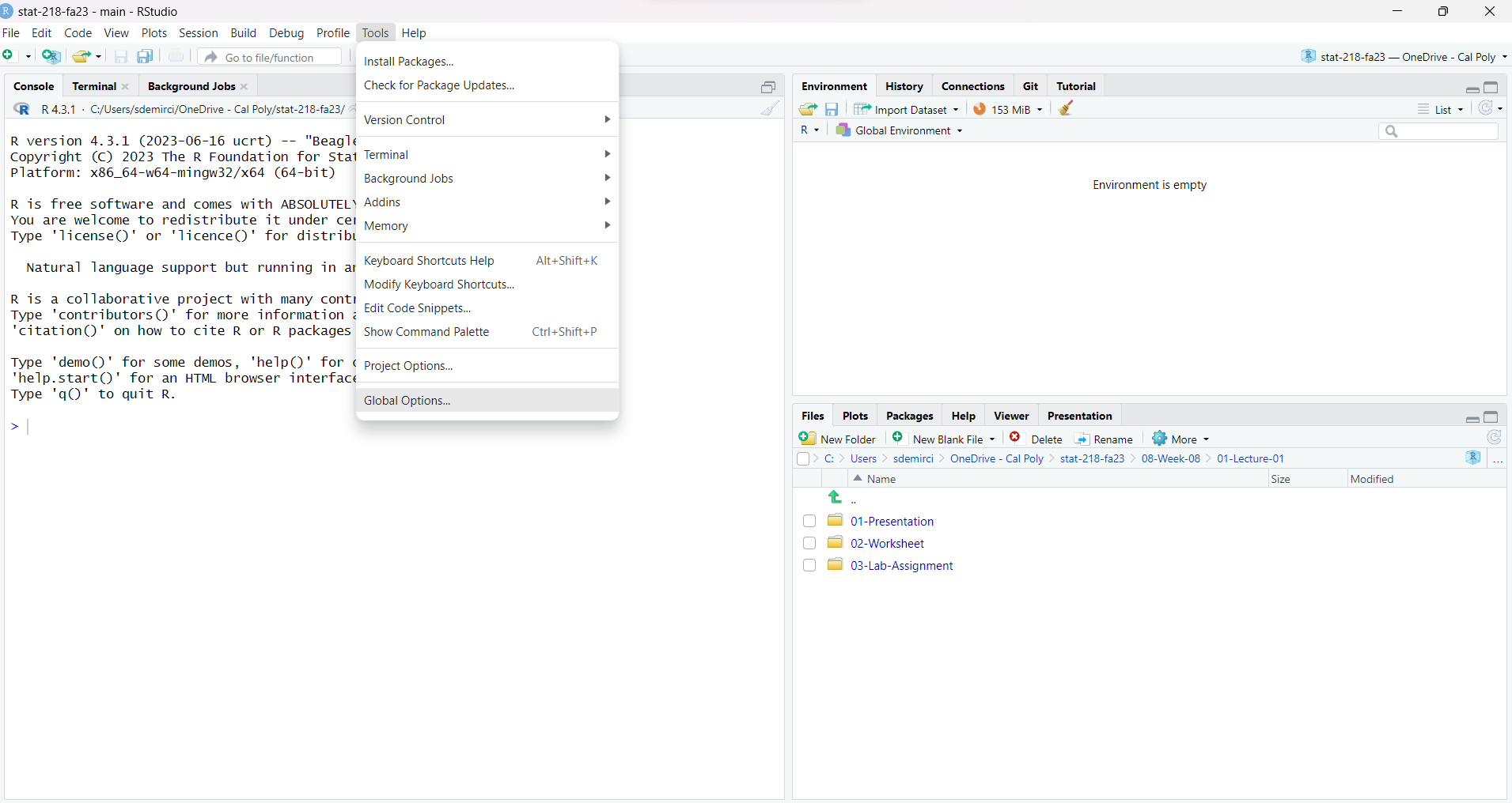
Before Proceeding Further…
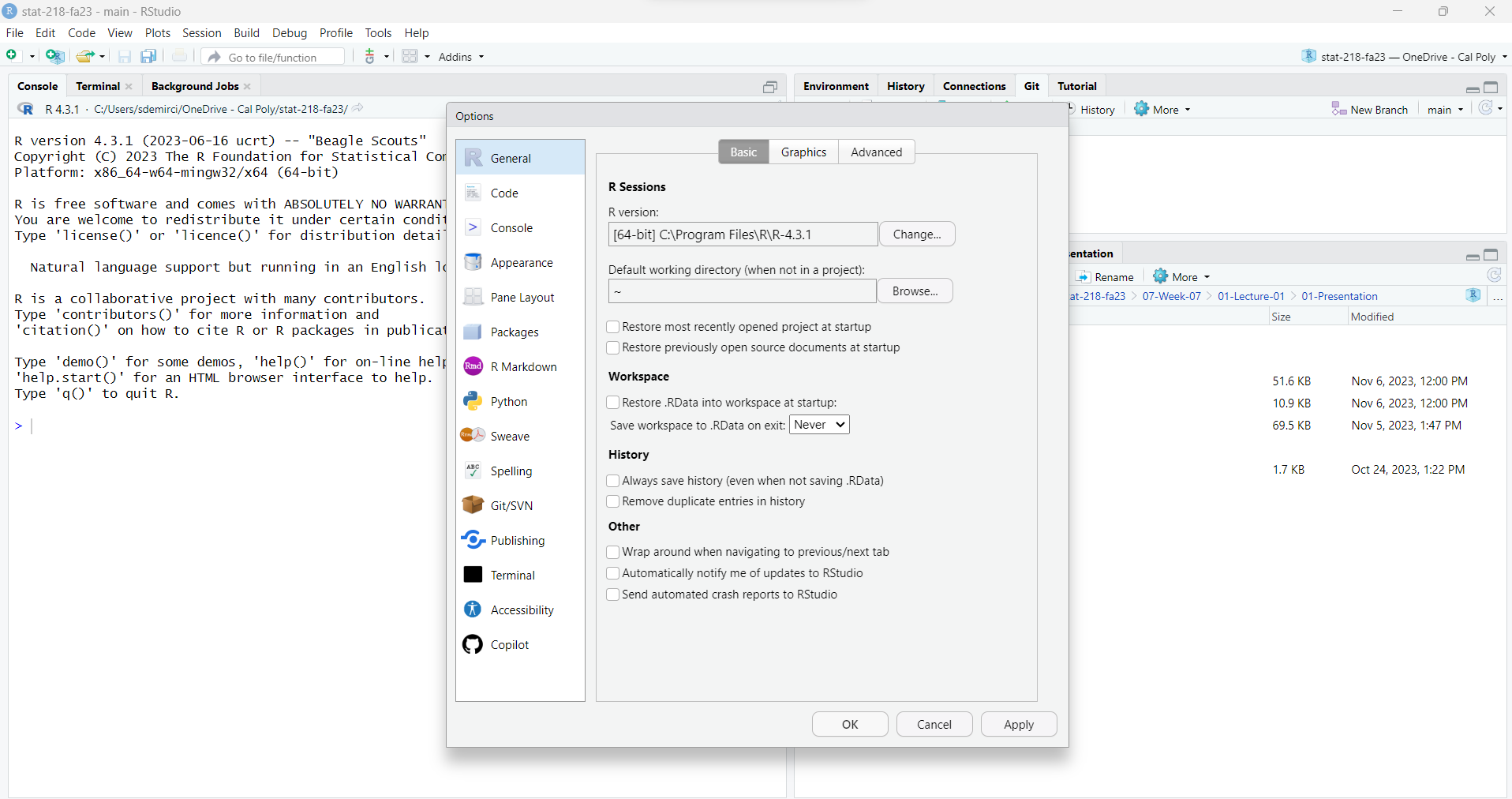
Today’s Menu
Today I will cover:
- more functions in R
- How to Install Packages
- Loading Data into R
- Summary Statistics
ggplot()
Then you will…
- download your assignment
- work in groups
- start your first assignment in R
A Quick note
Next slides are just for demonstration purposes. Please DO NOT code, just watch my demo.
I’ve created a Quarto document for you, you’ll download it after this demonstration.
After that, you will work with your group members.
You may not finish it today but you have time until Tuesday midnight.
Installing a Package
R users can create/contribute packages, and they are free!
For this lab, and many others in the future, we will use:
- The
tidyverse“umbrella” package which has many different R packages for data wrangling and data visualization - The
openintroR package is our second textbook’s package and we will use this for our lab sessions.
- The
AN ANALOGY: Packages are like toolboxes. You get them once and there’s no need to buy them over and over again. Once we install these packages, we can reuse them whenever we need.
The Library Function in R
The library() function in R is like opening a toolbox (Analogy continues).
When you use the library() function, you’re telling R to open a specific toolbox (load a package) so that you can access and use the tools inside.
If you don’t open the toolbox, you can’t use what’s inside. In the same way, you need to use the library() function every time you want to use a package (Analogy ends).
How to Load Data into R
We have two different ways to do that (within the scope of this class)
- Using an available dataset stored in R (packages) (we’ll do that today)
- Importing a dataset from an outside source (around Week 7-8)
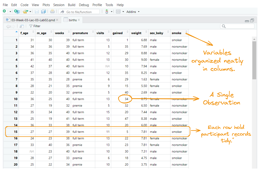
Getting to Know Your Data
After importing our data, it is important to familiarize with our data. We have some functions to do that.
I’ll start with glimpse() function. The name of this function is self-explanatory.
Rows: 150
Columns: 9
$ f_age     <int> 31, 34, 36, 41, 42, 37, 35, 28, 22, 36, 27, 35, 25, 36, 27, …
$ m_age     <int> 30, 36, 35, 40, 37, 28, 35, 21, 20, 25, 19, 34, 19, 33, 27, …
$ weeks     <int> 39, 39, 40, 40, 40, 40, 28, 35, 32, 40, 32, 40, 41, 38, 39, …
$ premature <fct> full term, full term, full term, full term, full term, full …
$ visits    <int> 13, 5, 12, 13, NA, 12, 6, 9, 5, 13, 5, 15, 13, 10, 11, 13, 1…
$ gained    <int> 1, 35, 29, 30, 10, 35, 29, 15, 40, 34, 32, 20, 47, 20, 5, 22…
$ weight    <dbl> 6.88, 7.69, 8.88, 9.00, 7.94, 8.25, 1.63, 5.50, 2.69, 8.75, …
$ sex_baby  <fct> male, male, male, female, male, male, female, female, male, …
$ smoke     <fct> smoker, nonsmoker, nonsmoker, nonsmoker, nonsmoker, smoker, …
Getting to Know Your Data
Rows: 150
Columns: 9
$ f_age     <int> 31, 34, 36, 41, 42, 37, 35, 28, 22, 36, 27, 35, 25, 36, 27, …
$ m_age     <int> 30, 36, 35, 40, 37, 28, 35, 21, 20, 25, 19, 34, 19, 33, 27, …
$ weeks     <int> 39, 39, 40, 40, 40, 40, 28, 35, 32, 40, 32, 40, 41, 38, 39, …
$ premature <fct> full term, full term, full term, full term, full term, full …
$ visits    <int> 13, 5, 12, 13, NA, 12, 6, 9, 5, 13, 5, 15, 13, 10, 11, 13, 1…
$ gained    <int> 1, 35, 29, 30, 10, 35, 29, 15, 40, 34, 32, 20, 47, 20, 5, 22…
$ weight    <dbl> 6.88, 7.69, 8.88, 9.00, 7.94, 8.25, 1.63, 5.50, 2.69, 8.75, …
$ sex_baby  <fct> male, male, male, female, male, male, female, female, male, …
$ smoke     <fct> smoker, nonsmoker, nonsmoker, nonsmoker, nonsmoker, smoker, …
glimpse() function gives us a brief information about out data set. We have 9 variables and 150 cases or observations.
Getting to Know Your Data
Alternatively, I can ask R the number of columns (variables) and rows (cases) as following:
[1] 9[1] 150Assume that I would like to see just the names of the variables in my data set. I can use names()function for this.
Frequency Distribution Table (An Ugly One!)
I’ll construct a frequency distribution table by using count()function.
Measures of Central Tendency
We can calculate measures of central tendency by using these unsurprising functions.
Pay attention to the $ sign.
Measures of Dispersion
Standard deviation
Measures of Central Tendency
Alternatively, I can use summarize() function for the same calculations.
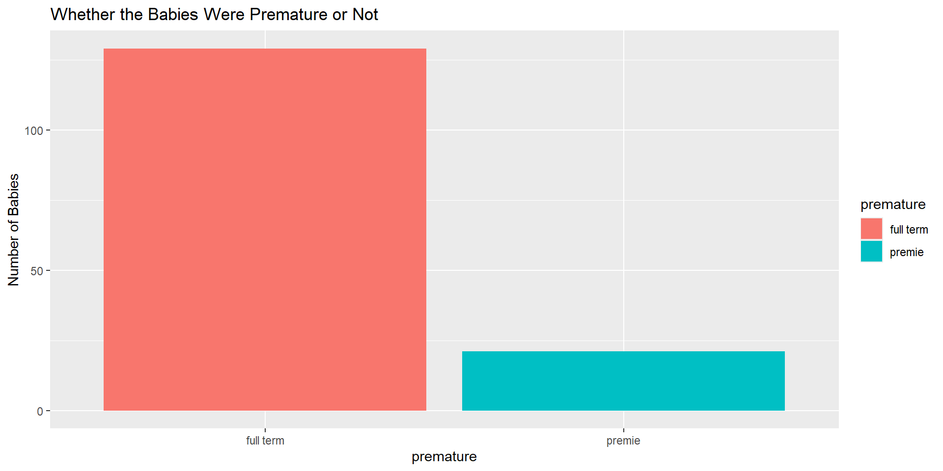
An Example for Bar Chart
I’ll plot a simple bar chart. Next session, we will explore other features for ggplot().
An Example for Bar Chart
I’ll plot a simple bar chart. Next session, we will explore other features for ggplot().
SUMMARY OF FUNCTIONS USED TODAY
How did these function work?
# Replace DATASET with the name of your dataset
# Replace VARIABLE with the variable you are analyzing

# Example:
# DATASET  -> births
# VARIABLE -> weight

data("DATASET")
glimpse(DATASET)
ncol(DATASET)
nrow(DATASET)
names(DATASET)
count(DATASET, VARIABLE)
mean(DATASET$VARIABLE, na.rm = TRUE)
median(DATASET$VARIABLE, na.rm = TRUE)
sd(DATASET$VARIABLE, na.rm = TRUE)
HOW CAN YOU STUDY WITH YOUR GROUP MEMBERS?
A SUGGESTION
To ensure the group’s work is divided equitably each week, your team will be rotating through a set of group roles. This ensures one person doesn’t act as the group leader for multiple sessions of class, while someone else is always the note taker. You will circulate through the following roles each week:
Project Manager:
- Coordinate the group’s activities, ensuring tasks are assigned and deadlines are met.
- Facilitate communication within the group and with the instructor.
- Ensure the final assignment is compiled and submit it.
Note Taker:
- Responsible for interpreting and documenting the outputs generated from R scripts/codes.
- Take notes on key findings, insights, and interpretations derived from the data and analyses.
Coder:
- Lead the coding efforts, writing and managing the R scripts.
- Ensure code quality, functionality, and documentation standards are met.
A SUGGESTION
If you work in pairs, skip the project manager role ans switch coding/note-taking every week.
Note takers should either take notes to a paper or a Word document and add them later to the quarto document once coding part finished.
Your Turn
Today’s Quarto Document
Tip
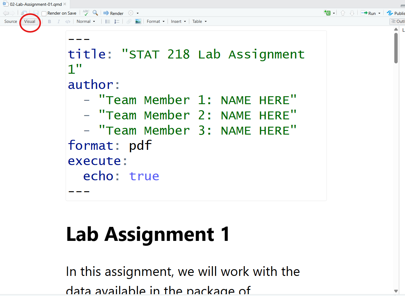
- Let’s download today’s Quarto document from Canvas under the LAB Assignment 1 (GROUP) titled as
02-Lab-Assignment-01.qmd - DO NOT FORGET to save it to your STAT 218 Folder!
Also…
Do not forget to open “Visual” Mode.
How to Complete Lab Assignment 1
Just go back and follow this slide show from the beginning of Slide 10.
You will be mainly changing the name of the data set and variables.
Call me over if you have any questions.