Independent Samples t-test and Confidence Interval

Today’s Menu

• A quick review of the confidence interval for a single mean
  
• Independent samples t-test
• Confidence interval for the difference of two population means
  
• Revisiting confidence interval interpretations from the concept cartoon (if we have time)

Introduction

• In practice, most of the scientific research involves the comparison of 2 or more samples from different populations.

• Today, we will be dealing with the comparison of 2 means

Interval Estimation for A Single Mean

Let’s Refresh Our Memory

• Confidence interval is an interval of plausible values for the parameter of interest.

• A parameter is a (fixed but typically unknown) number that describes a population.

What is the general form of a confidence interval for a parameter?

\[ statistic \pm (estimated) \ margin \ of \ error \]

\[ \\statistic \pm multiplier \times estimated \ SD \ of \ statistic \]

Confidence Interval for a sample mean is…

\[ \\ \bar{x} \pm t^*_{df} \ \times \ \frac{s}{\sqrt{n}} \]

Let’s Revisit Monarch Butterflies Example

Let’s assume that we examined the wing areas of 92 Monarch butterflies (Danaus plexippus) from the eastern North American population (df = 91 and multiplier obtained from software: \(t^*\) = 1.99)

\(n = 92\), \(\bar{x} = 33.36\) \(cm^2\) and \(s= 2.22\) \(cm^2\)

95% confidence interval (CI) for \(\mu\) is:

\[ \\ \bar{x} \pm t^*_{df} \ \times \ \frac{s}{\sqrt{n}} \\ 33.36 \pm 1.99 \ \times \ \frac{2.22}{\sqrt{92}} \]

\[ \\ 95 \% \ CI = (32.90,\ 33.82) \]

Interpretation:

We are 95% confident that the population mean wing area of Monarch butterflies from eastern North America is between 32.90 \(cm^2\) and 33.82 \(cm^2\).

What Is Next?

Interval Estimation for the Difference of Two Population Means

Step 1. Understanding the Study

In the previous example, we estimated the population mean wing area for Monarch butterflies from eastern North America using a sample of 92 butterflies.

We now use the same real study to estimate the difference in population mean wing area between male and female butterflies, \(\mu_{m}\) − \(\mu_{f}\).

\(n_m = 47,\ \bar{x}_m = 33.87 \ \text{cm}^2,\ s_m = 2.22 \ \text{cm}^2\)

\(n_f = 45,\ \bar{x}_f = 32.84 \ \text{cm}^2,\ s_f = 2.12 \ \text{cm}^2\)

Let’s first identify these:

observational unit, variable(s), parameter, statistic

Step 2. Study Design

Observational unit: A Monarch butterfly

Explanatory variable: Male/Female (Categorical - Binary)

Response variable: Wing area \((cm^2)\)

Statistical Study Type: Observational study

Randomization: Although the original study did not mention explicitly, we will assume that the sample is representative of all butterflies in the population.

Statistic: the observed difference in sample mean wing areas between male and female butterflies \(\bar{x}_m\) − \(\bar{x}_f\).

Parameter: the difference in population mean wing areas between male and female butterflies \(\mu_{m}\) − \(\mu_{f}\). (Remember this is an unknown fixed value.)

Step 3: But First… Explore the Data

Validity Conditions: The quantitative variable should have either

• a symmetric distribution in both groups, or

• at least 20 observations in each group and the sample distributions should not be strongly skewed.

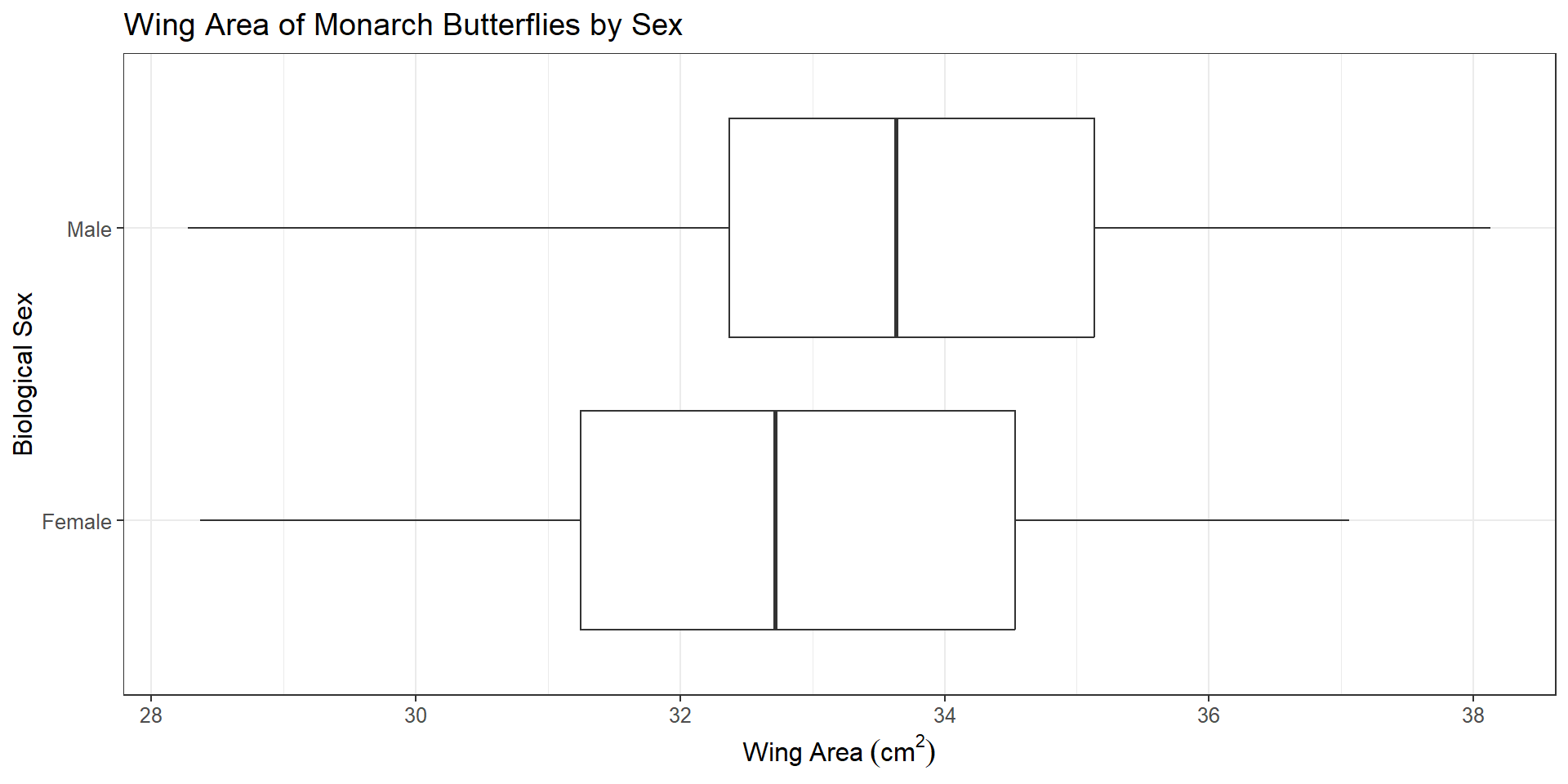
\(n_m = 47,\ \bar{x}_m = 33.87 \ \text{cm}^2,\ s_m = 2.22 \ \text{cm}^2\)

\(n_f = 45,\ \bar{x}_f = 32.84 \ \text{cm}^2,\ s_f = 2.12 \ \text{cm}^2\)

Remember: boxplots help us identify the presence of strong skewness

Step 4. Draw Inferences - Hypothesis Testing and Confidence Interval

The Null and Alternative Hypotheses

The hypothesis that \(\mu_1\) and \(\mu_2\) are not equal is called an alternative hypothesis (or a research hypothesis)

\[ H_A: \mu_1 \neq \mu_2 \]

Its antithesis is the null hypothesis, \[ H_0: \mu_1 = \mu_2 \]

which asserts that \(\mu_1\) and \(\mu_2\) are equal. A researcher would usually express these hypotheses more informally and we can trace those hypotheses from the examples, problems and exercises in this course.

Alternatively we can express these hypotheses as following:

\[ \\H_0: \mu_1 - \mu_2 = 0 \\H_A: \mu_1 - \mu_2 \neq 0 \]

Calculate test statistic

• Test statistic is a measure of how far the difference between the sample means (\(\bar{x}\)’s) is from the difference we would expect to see if \(H_0\) were true (zero difference), the amount of variation we expect to see in differences of means from random samples.

\[ test \ statistic = \frac{(\bar{x}_1 - \bar{x}_2) - (\mu_1 - \mu_2)}{SE(\bar{x}_1 - \bar{x}_2)} \]

But What is Standard Error?

The formula that we have used so far is

\[ SE_{\bar{X}} = \frac{s}{\sqrt{n}} \]

• Naturally, we can say that taking the difference between two sample means is an estimate of the quantity (\(\mu_1\) - \(\mu_2\)).

• However, the formula for the standard error of the difference (\(\bar{X}_1\) - \(\bar{X}_2\)) is a little different from what we initially thought.

\[ SE_{\bar{X}_m - \bar{X}_f} = \sqrt{SE_m^2 + SE_f^2} \]

\[ SE_{\bar{X}_m - \bar{X}_f} = \sqrt{ \frac {s_m^2}{n_m} + \frac {s_f^2}{n_f}} \]

\[ SE_{\bar{X}_m - \bar{X}_f} = \sqrt{ \frac {2.22^2}{47} + \frac {2.12^2}{45}} ≈ 0.452 \]

Calculate test statistic

\[ test \ statistic = \frac{(\bar{x}_1 - \bar{x}_2) - (\mu_1 - \mu_2)}{SE(\bar{x}_1 - \bar{x}_2)} \]

\[ \frac{(33.87 - 32.84) - (0)}{0.452} ≈ 2.28 \ (??) \]

Parameter Estimation - Confidence Interval

General form of a confidence interval for a parameter

\[ \\statistic \pm (estimated) \ margin \ of \ error \]

\[ statistic \pm multiplier \times \ estimated \ SD \ of \ statistic \]

Let’s specify that for comparing two means.

\[ \\ (\bar{x}_m - \bar{x}_f) \pm t^*_{df} \ \sqrt{\frac{s_m^2}{n_m} + \frac{s_f^2}{n_f}} \]

Step 4. Parameter Estimation

95% Confidence Interval for \(\mu_{m}\) − \(\mu_{f}\). (multiplier obtained from software: \(t^*\) = 1.99)

\(n_{m}=47\) \(\bar{x}_m = 33.87\) \(cm^2\) and \(s_m= 2.22\) \(cm^2\)

\(n_{f}=45\) \(\bar{x}_f = 32.84\) \(cm^2\) and \(s_f= 2.12\) \(cm^2\)

\[ \\ (\bar{x}_m - \bar{x}_f) \pm t^*_{df} \ \sqrt{\frac{s_m^2}{n_m} + \frac{s_f^2}{n_f}} \\ \\ (33.87 - 32.84) \pm 1.99 \ \sqrt{\frac{2.22^2}{47} + \frac{2.12^2}{45}} \\ \\ 1.03 \pm 0.899 \]

95% CI for difference in population means = (0.131, 1.929)

Interpretation: We are 95% confident that the population mean wing area for male Monarch butterflies is between 0.13 cm² and 1.93 cm² higher than that for female Monarch butterflies in eastern North America.

R, Please Save Me!

t_test(x = mydata, 
       formula = wing_area_cm2 ~ sex, 
       order = c("Male", "Female"),
       alternative = "two-sided",
       var.equal = FALSE)

# A tibble: 1 × 7
  statistic  t_df p_value alternative estimate lower_ci upper_ci
      <dbl> <dbl>   <dbl> <chr>          <dbl>    <dbl>    <dbl>
1      2.28  90.0  0.0252 two.sided       1.03    0.131     1.93

More on Confidence Interval

• This interval contains only positive values and does not contain 0.
  • Thus, we have convincing statistical evidence that the difference in mean wing areas between male and female Monarch butterflies is not 0.
  • More specifically, we are 95% confident that the population mean wing area for male Monarch butterflies is between 0.13 cm² and 1.93 cm² higher than that for female Monarch butterflies in eastern North America.

• If nothing else changes when comparing two means, will the confidence interval be narrower/wider? if we:
  • increase the sample size,
  • increase the confidence level, or
  • decrease the data variability (standard deviation)

What Does “95% Confident” Mean, Again?

Student D

This is a typical misconception. Confidence interval shows a range of plausible values that applies to population means, not individual butterflies.

It gives us a range within which we believe the true difference in population mean wing area between male and female Monarch butterflies lies, not where individual wing areas fall.

Student C

Actually, we know for 100% certain that the sample statistic is the midpoint of the confidence interval.

\[ \\ (\bar{x}_m - \bar{x}_f) \pm t^*_{df} \ \sqrt{\frac{s_m^2}{n_m} + \frac{s_f^2}{n_f}} \]

Student A

This is another misconception too.

• Remember, the parameter is a fixed value. The confidence interval either contains the true difference in population mean wing area or it does not.

• Hence, the words like ‘probability’ or ‘chance’ are not technically relevant to this particular interval.

But What Does “95% Confident” Mean?

Understanding Confidence Intervals

It is about the long-run performance of the method.

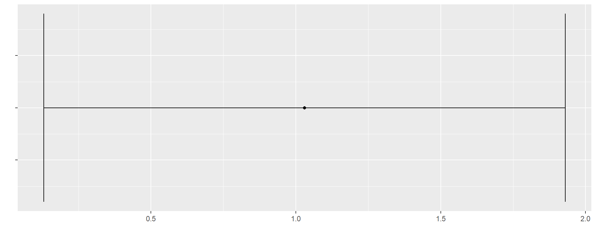
This is the 95% CI we found as (0.13, 1.93) in the previous question.

Understanding Confidence Intervals

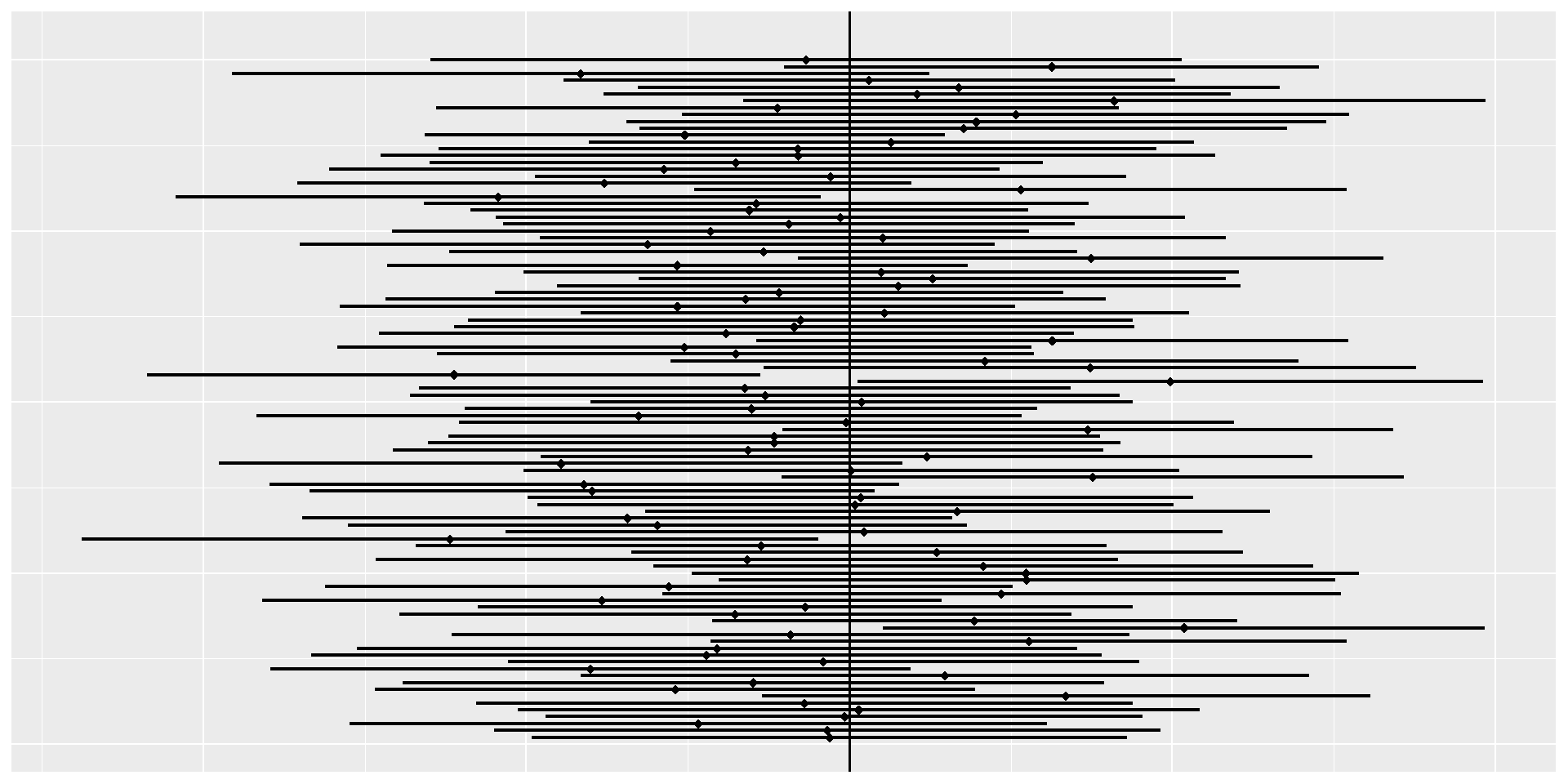
What would happen to the confidence intervals if we repeated this study 100 times with new random samples?

Understanding Confidence Intervals

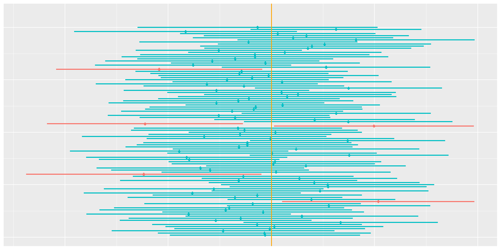
About 95 of those intervals would contain the true difference between the two population means (assuming the vertical line represents the true parameter).

Understanding Confidence Interval

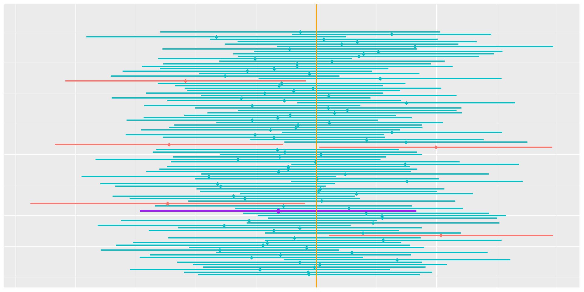
Normally, we wouldn’t know whether our CI was red or blue but our confidence interval might be this?

Understanding Confidence Interval

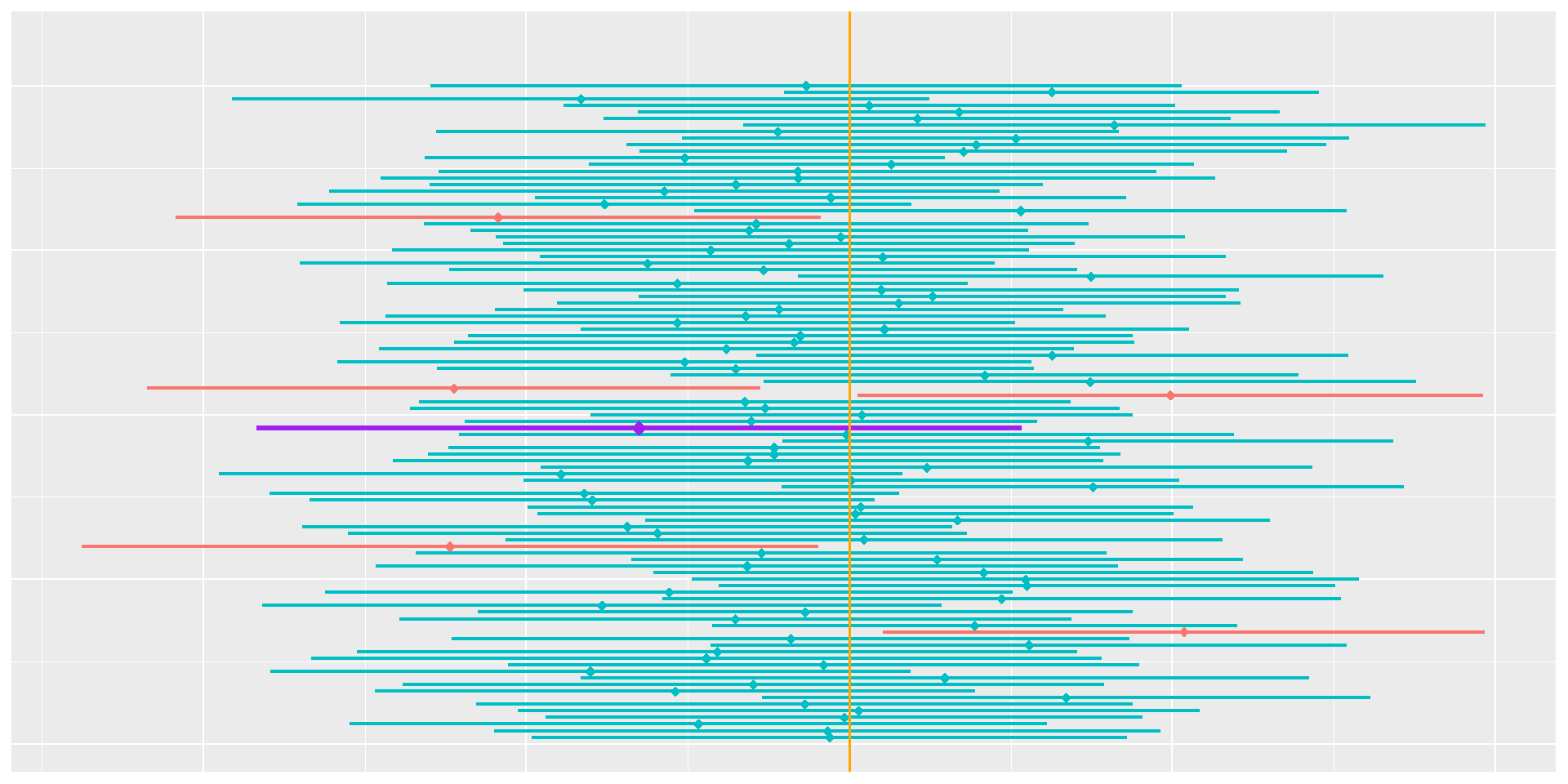
Or this?

Student B - Correct Answer

We are 95% confident that the population mean wing area for Monarch butterflies is between 0.13 cm² and 1.93 cm² higher than that for female Monarch butterflies in eastern North America.

Over many repeated samples, this method captures the true population parameter about 95% of the time.

Key Takeaways

• Confidence interval for (\(\mu_1 \ - \mu_2\)) gives an interval of plausible values for the difference in population means.

• Pay attention to whether the confidence interval is entirely positive or negative, or includes 0.

• Always check validity conditions before constructing and interpreting a confidence interval.