Ch. 6 & Ch. 7: Review of \(t\)-tests

STAT 218 - Week 6, Lecture 4 Lab 3

What Have We Learned So Far?

A Snapshot

Inferential Statistics makes predictions and draws conclusions about populations based on sample data.
- We saw different types of t-tests:
  - One sample t-test: compares a sample mean to a known or hypothesized population mean.
  - Independent samples t-test: compares means of two independent groups.
We’ll see these tests today.

Hypothesis Testing Steps

Introduction

Important

We can summarize hypothesis testing in four steps (if we use theory-based approach):

Construct the Hypotheses of \(H_0\) and \(H_A\).
Check the validity conditions/assumptions
Compute test statistic, find the p-value and confidence interval (Interpreting R Output)
Draw conclusion.

To-do List Before Start - I

Assign your roles.

Project Manager:

Follow the slides and give directions to the coder and note taker.
Facilitate communication within the group and with the instructor.

Note Taker:

Take notes on key findings, insights, and interpretations derived from the data and analyses.

Coder:

Lead the coding efforts, writing and managing the R scripts.
Ensure code quality, functionality, and documentation standards are met.

To-do List Before Start - II

Download the assignment from course website (Lab Assignment 3).
Follow the instructions on this slideshow to complete the assignment.

Setting the Scene

Downloading Necessary Packages

To begin with, we need infer package to conduct t tests.
Let’s run the code chunk in our lab assignment 3 file and load infer package by using install.packages() function.

install.packages("infer")

Running Library Functions and Loading Datasets

After loading that package, let’s run library functions and load the data set that we will use today.

library(tidyverse)
library(infer)
library(palmerpenguins)
data("penguins")

One Sample \(t\)-test

Example of a Case:

Imagine that you are a biologist studying penguins, particularly their bill lengths. Previous studies have hypothesized that the population mean bill length of penguins is 40 mm. You collect a random sample of 344 penguins and measure and record their bill lengths in millimeters.

Perform a one sample \(t\)-test to investigate whether the bill length of the penguins differs from the test value of 40 mm.

Instructions

Open the assignment file and answer the following questions.

Question 1. What is the research question of this study?

Type your answer in the assignment file.

Question 2. What type of variable is used in this study?

Type your answer in the assignment file.

Assumptions - Validity Conditions

It is always important to check first whether the conditions are reasonable in a given case.
Here is the list of conditions that we should be aware of for one sample \(t\)-test.

1) Random Sampling: the data can be regarded as coming from independently chosen random sample,

2) Independence of Observations: the observations should be independent (One observation does not influence another.). If (1) You randomly sample individuals from a very large population, and (2) Each selection does not affect another, then observations are typically independent.

3) Normality Assumption: You should have either symmetric (approximate normality) population distribution
OR
n > 30 (some references says 20) AND sample distribution not strongly skewed.

Normality Assumption - I

If the only source of information is the data at hand, then normality can be roughly checked.
- Unfortunately, for a small or moderate sample size, this check is fairly rudimentary.
- If the sample is large, then the visual plots (histogram) give us good information;
  - However, if \(n\) is large, the requirement of normality is less important anyway due to the Central Limit Theorem.
In any case, a rudimentary check is better than none, and every data analysis should begin with inspection of a graph of the data, with special attention to any observations that lie very far from the center of the distribution.

Question 3. Checking the Normality Assumption

Check your sample size first!
- sample size is large, so we can check visual plots.
Direction: Please create a histogram to check the normality.

Question 4. Interpreting the Output

t_test(penguins, response = bill_length_mm, mu = 43)

# A tibble: 1 × 7
  statistic  t_df p_value alternative estimate lower_ci upper_ci
      <dbl> <dbl>   <dbl> <chr>          <dbl>    <dbl>    <dbl>
1      3.12   341 0.00194 two.sided       43.9     43.3     44.5

Conclusion: Type your hypothesis testing conclusion to your assignment file!

Confidence Interval: Type your confidence interval statement to your assignment file!

Independent Samples \(t\)-test

Example of a Case:

Now, you’re curious about the difference in the body mass of penguins based on their sex. You hypothesize that body mass varies between different sexes. To test your hypothesis, you collect a random sample of 344 penguins, measure their body mass, and record their sex.

Perform an independent samples \(t\)-test to investigate whether the body mass of penguins differs between different sexes.

Instructions

Continue with the assignment file and answer the following questions.

Question 1. What is the research question of this study?

Type your answer in the assignment file.

Question 2. What type of variable is used in this study?

Type your answer in the assignment file.

Assumptions - Validity Conditions

It is always important to check first whether the conditions are reasonable in a given case.
Here is the list of conditions that we should be aware of for independent samples \(t\)-test.

1) Random Sampling: the data can be regarded as coming from independently chosen random sample(s),

2) Independence of Observations: the observations should be independent (One observation does not influence another.).If (1) You randomly sample individuals from a very large population, and (2) Each selection does not affect another, then observations are typically independent.

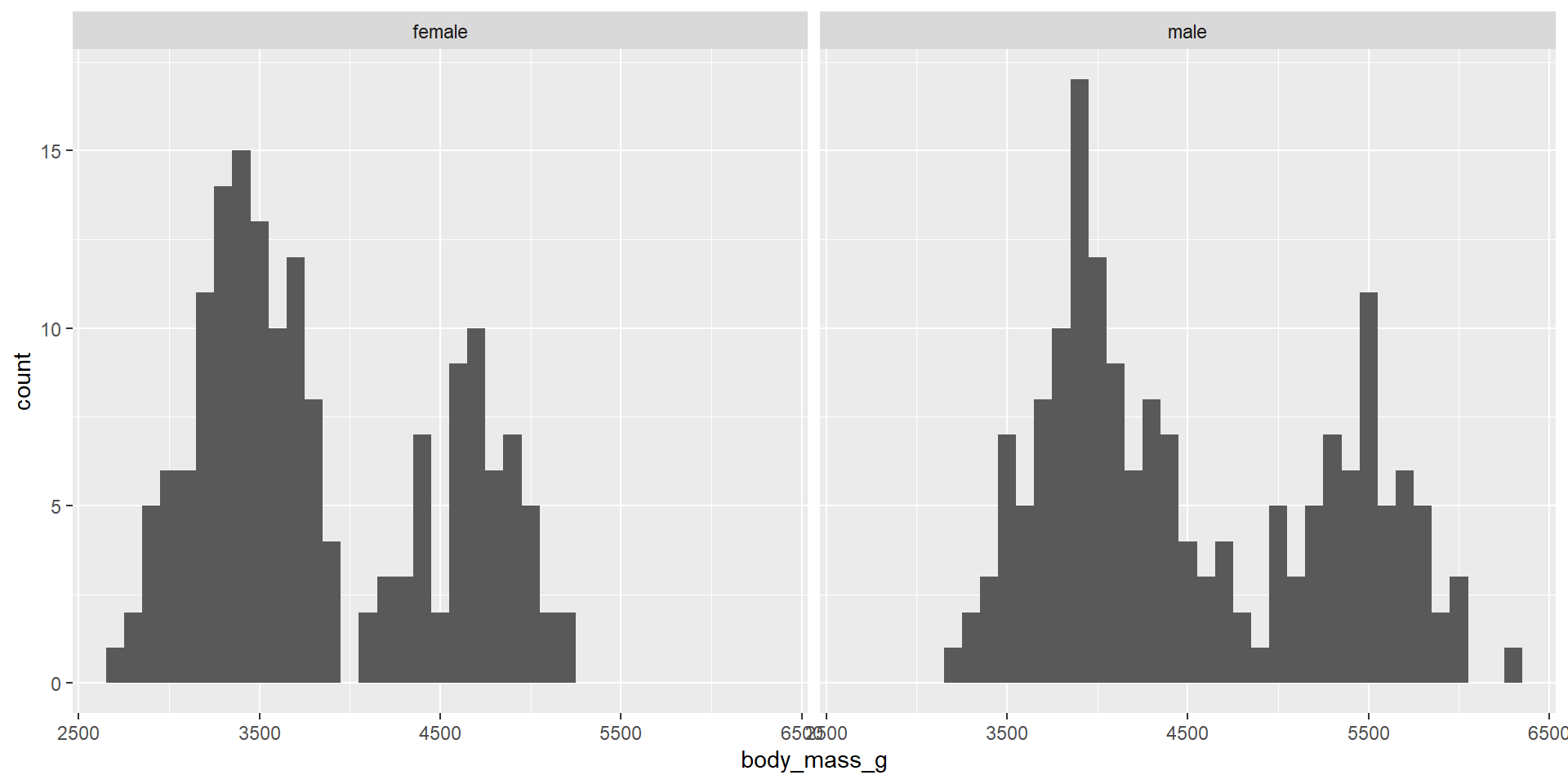
3) Normality Assumption: n > 20 for each group AND sample distributions should not be strongly skewed.

Question 3. Checking the Normality Assumption

Check your sample size first!
- sample sizes are large, so we can check visual plots (e.g., histogram) for each group.

Question 3. Creating Two Histograms for Normality

ggplot(data = na.omit(penguins),
       aes(x = body_mass_g)) +
  geom_histogram(binwidth = 100) +
  facet_wrap(~sex)

Question 4. Interpreting the Output

t_test(x = penguins, 
       formula = body_mass_g ~ sex, 
       order = c("male", "female"),
       alternative = "two-sided",
       conf_level = 0.90)

# A tibble: 1 × 7
  statistic  t_df  p_value alternative estimate lower_ci upper_ci
      <dbl> <dbl>    <dbl> <chr>          <dbl>    <dbl>    <dbl>
1      8.55  324. 4.79e-16 two.sided       683.     552.     815.

Conclusion: Type your hypothesis testing conclusion to your assignment file!

Confidence Interval: Type your confidence interval statement to your assignment file!