Paired \(t\)-test

STAT 218 - Week 7 Lab 4

Let’s Remember Hypothesis Testing Steps

Revising the Steps of Hypothesis Testing

Important

1. Construct the Hypotheses of \(H_0\) and \(H_A\)
2. Check the assumptions
3. Compute test statistic and find the p-value (Interpreting R Output)
4. Draw conclusion.

To-do List Before Start - I

• Assign your roles.

Project Manager:

• Follow the slides and give directions to the coder and note taker.
• Facilitate communication within the group and with the instructor.

Note Taker:

• Take notes on key findings, insights, and interpretations derived from the data and analyses.

Coder:

• Lead the coding efforts, writing and managing the R scripts.
• Ensure code quality, functionality, and documentation standards are met.

To-do List Before Start - II

1. Download the assignment from Canvas (Lab Assignment 4).
   
2. Download the dataset from Canvas.
   

• Mac Users: Downloading a .csv file from Canvas can be tricky. Try opening it in a new tab to download.
• Windows Users: Congratulations, you are privileged and blessed! Your .csv file should download without a fight (hopefully).
  
• Important: Even if you manage to download it, please do not open it on your computer. Mac sometimes automatically changes the file extension (yes, really!), which makes it harder to import with this lab’s code.

3.Save both files to your STAT 218 folder (VERY IMPORTANT). Otherwise, you won’t be able to import the dataset.
4. Ensure your assignment and dataset are in the same folder, with file extensions .qmd and .csv.
5. Follow the instructions on this slideshow to complete the assignment.

Running Library Function and Loading Dataset

Let’s run library functions and load the data sets that we will use today.

library(tidyverse)
stream <- read_csv("stream.csv")

IMPORTANT!: If you don’t see stream in your Environment Pane, this means that your dataset and quarto file are not in the same folder! CALL ME OVER!

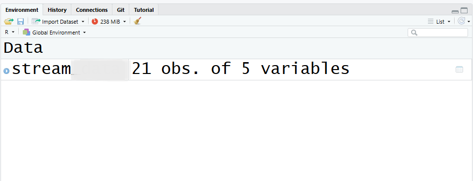
OR…

You may have downloaded stream.csv multiple times, so its name could look like stream (2)(1).csv.

Check the file name, correct it if necessary, and try again. Remember, R is very stubborn—it won’t read the data if the name doesn’t match exactly what you typed in your code.

Paired Samples \(t\)-test

Example of a Case: Pollutants in a stream may accumulate or attenuate as water flows down the stream. In a study to monitor the accumulation and attenuation of fecal contamination in a stream running through cattle rangeland, monthly water specimens were collected at two locations along the stream over a period of 21 months.

The data set stream the total coliform count (MPN/100ml) for a water specimen.

Perform a paired sample \(t\)-test to assess whether the mean total coliform count is consistent across the two locations.

Assumptions - Validity Conditions

• It is always important to check first whether the conditions are reasonable in a given case.

• Here is the list of conditions that we should be aware of for paired sample \(t\)-test.

1) Random Sampling: The pairs (or subjects) should come from a random sample OR The treatment conditions should be randomly assigned (in experiments),

2) Independence of Observations: the pairs should be independent of other pairs (One subject’s pair of measurements should not influence another subject’s pair.).

⚠️ Important distinction:

Measurements within a pair are NOT independent (that’s why we use a paired test).

But the pairs themselves must be independent.

3) Normality of the Differences: At least 20 pairs (i.e., at least 20 differences) and the distribution of the sample differences is not strongly skewed.

Checking the Normality Assumption

• Check your sample size first!

  • Relatively small, so we should check Shapiro-Wilk test.

• Shapiro–Wilk Test is a statistical method that provides a numerical assessment of evidence for certain types of nonnormality in data.

  • The procedure’s mechanics are complex, but statistical software packages simplify the testing process. Output and Interpretation:

• The output of the Shapiro–Wilk test includes a P-value. Interpretation:

  • P-value < 0.001: Very strong evidence for nonnormality.
  • P-value < 0.01: Strong evidence for nonnormality.
  • P-value < 0.05: Moderate evidence for nonnormality.
  • P-value < 0.10: Mild or weak evidence for nonnormality.
  • P-value > 0.10: No evidence for nonnormality.

• This output is from a calculation of Shapiro-Wilk test. We generally use Shapiro-Wilk test for relatively smaller sample size because visuals can be misleading in smaller sample sizes. Please interpret Shapiro-Wilk \(p\)-value.

Shapiro-Wilk normality test

data: stream$Difference W = 0.9641, p-value = 0.6022

t_test vs. t.test

• If you notice, we used t_test() function so far while conducting independent samples t-test by using infer package.

• Now, we will use t.test() which is available default in R (And some BIO courses use this too).

Interpreting the Output - Question 4.2

t.test(stream$upstream, stream$downstream, paired = TRUE)

    Paired t-test

data:  stream$upstream and stream$downstream
t = 4.6092, df = 20, p-value = 0.0001697
alternative hypothesis: true mean difference is not equal to 0
95 percent confidence interval:
  603.7724 1602.0562
sample estimates:
mean difference 
       1102.914 

Interpreting the Output - Question 4.3

t.test(stream$difference, mu = 0)

    One Sample t-test

data:  stream$difference
t = 4.6092, df = 20, p-value = 0.0001697
alternative hypothesis: true mean is not equal to 0
95 percent confidence interval:
  603.7724 1602.0562
sample estimates:
mean of x 
 1102.914 

Question 4.4

Compare and contrast how the codes in Question 4.2 and Question 4.3 work. Comment on the

• p-value,
• test statistic, and
• confidence interval.

If they produce the same results, explain what the two codes did differently.

t.test(stream$upstream, stream$downstream, paired = TRUE)

t.test(stream$difference, mu = 0)

Question 4.5

Conclusion: Type your conclusion statement to your assignment!

Confidence Interval: Type your confidence interval statement to your assignment!